In an age of generative design a heat map can give a human perhaps a different kind of insight.
A heat map is as a surface with a colored gradient. And the colors represent a value, or even a wright and a wrong. The nice thing about a colored gradient is that the computer does the interpolation based on the actual calculated values. Off course in real life some of those values are not valid. And of course it is a very rough way to make decisions. But it does give some visual feedback. And it is based on calculations and not rules of thumb.
So let’s do this!. And make some heat maps in Dynamo and Revit. See what happens. And what works.

First Dynamo
For a heat map you first need a surface. So let’s select a Face from an object in Revit.
Now the first thing you need to know about generating a heat map in Dynamo is that you need a matrix (list of list) of points. The list of list must be with the same lengths and offsets. So in normal language. Create a bounding box based on the surface. Convert this into real geometry. Explode this to grab the bounding surface. And that is where we are going to work with. We divide this new surface into points. This can easily be done with Surface.PointAtParameter based on a UV. Both the U and the V are lists between 0 and 1 with equal steps for both in the U and in the V directions. The UV is like the local coordination system for the new heat map. The generating heat map needs this environment to work correct in Dynamo. Some points are on the Surface and some are not. This works differently in Dynamo and in Revit. But we will get back on that later.
So we have a surface and a list of list of points. Based on a bounding UV system.

Now let’s make Dynamo work!
Just for starters we will calculate the distance between each of these points and another object in Revit. In order to map each value to a colour in a color range between 0 to 1, we also need to map all the values between 0 and 1. Now we can find the right color for each value with the Color Range Node. At this moment each distance has a corresponding color. And this color is related to a UV position on the bounding surface because of the list structure. So when we connect this list of list of colors to the surface. We get a correct heat map. Points outside the surface do not matter for the GeometryColor.BySurfaceColors Node. Actually this Node needs all the UV points of the 2D bounding box to work correctly.

When we move the object in Revit the heat map in Dynamo will change. Nice… :-)
Off course we can also tweak the color range a little. The indices do not to be equally divided between 0 and 1. As long as there are as many colors as indices it will continue to work.

Because it is still a list of list with values. You can do some simple math and relate multiple heat maps to each other. Like the points nearest to object 1 AND object 2. Or the points nearest to object 2 and greatest distance to object 1. Off course this examples are not really difficult. I simply show how this works.

Now let’s take this heat map to Revit.
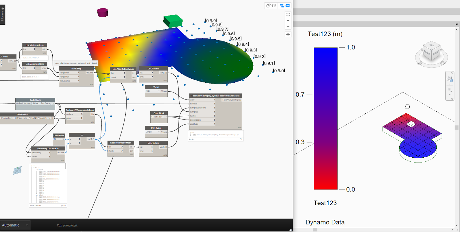
If we want to use the same points and values to create a heat map in Revit it does not work. We need to filter for points that are actually on the surface. This is the first thing that is different. And another thing is that we need a flatten list.


Of course Revit has its own View Visibility settings that also need to be correct to show the heat map. We need to create (or select) a Graphic Display Style – you can try different settings-. Be sure that Analysis Result Settings are also set. Also be sure that your kind of view is able to show the heat map –like 3D views-
Back to Dynamo.
There is more we can do while visualizing our calculated data. What about getting the contour of an area that is better (or worse) than a specific value? That is an interesting concept, I think. Because In the end you want the computer to understand that we are pinpointing things to a specific area that make sense. Jus in order to (visually) lower the endless combinations in front, while doing some generative design.
It gives us also other ways to visually or mathematically examine our results. Like the value at a specific point, based on interpolation. Or the slope – the difference between values in an bigger or smaller area. There are times that you best can generate millions of options –because it is simply too difficult to explain or program- And there are times when you are trying to find an optimum between the latest and doing things completely manually.


Create a solid while using the perimeter curves of the original surface and the new top surface.
And finally slice this new solid at a certain level.
Now we have a new piece of geometry that is roughly defined by calculations off a grid of points and a value filter. The slicer is not really fast... but it works.

Of course this is not all new.
ArchiLab has also some nodes. Here is an old post where he is playing with LadyBug and Mantis Shrimp
And then there is the SpaceAnalysis Package. Build by Autodesk Research. A package that can do some efficient tricks just out of the box. It has some wonderful solutions for Pathfinding (better than calculating the straight line distance in our example)), Visibility / Field of view and Acoustics.

I am happy to say that it is not really difficult to use. First you have to make a Space Lattice with the Node SpaceLattice.ByBoundingBoxAndLines. This node needs a bounding box (now you know), some barriers (real barriers, or the contour of the surface, or an empty list – but why would you) It is possible to enter a list of Revit lines, but also line based Revit families. Remember that curved lines do not work. In that case use Utils.ApproximateCurvesWithLines. And last but not least a resolution input. Take care of this one! This is a distance input and the default value is 0,2. Beware! Your script will probably not break. And when this node is finally finished you have a very detailed Space Lattice. When you first try this workflow make this input bigger than the default. Or try something like I did to reduce the points.

There are a few nodes that will show this Space Lattice. It contains of a grid of points. And all the points are connected with lines in maximum 8 directions. By walking and counting these lines you will have an idea how far points are apart. Especially if you see that the Space Lattice does not make these lines if they intersect with your barriers. Well in the end the shortest path is a fundamental science problem. Google Dijkstra’s algorithm if you are up to it. It can be fun to know at least some basics.
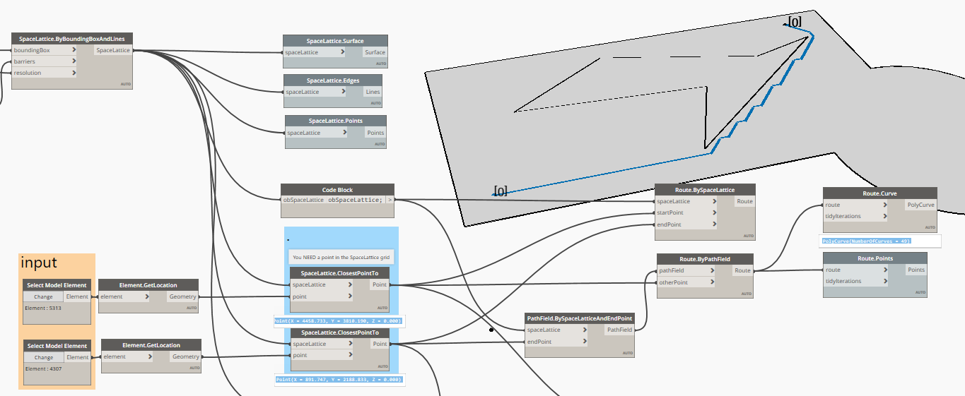
Because of this Space Lattice, you have to relate your input points to this Space Lattice with the node SpaceLattice.ClosestPointTo. At least that is what I think is best.

It is easy to find and visualize the shortest path. A nice addition is the tidyIteration to make the path more smooth. You probably want to do this if you do not use so much calculating points.

The field of view is only a few nodes. Here it is also possible to relate multiple results by using Union and Intersection. And there is also a node to get the value at a specific point.
Of course you need to do some tricks to get this visual into Revit, as described above.
Here you can find the scripts SpaceAnalysis_test.dyn and Heat_map_test.dyn so you play around.


